8. The Computational Toolbox
This section describes the specific software tools that are to be built. It should be viewed as a concept document not a requirements document. The discussion of each tool is brief, and comments are added about existing infrastructure that can be used to build each tool.
Many of the tools should work equally well with ground-based data or data from space observatories, but there is a need to include tools for standard kinds of ground-based data analysis. These are included, although the list may be less complete than for the JWST tools.
The figure below provides birds-eye view of the tools described in this section.
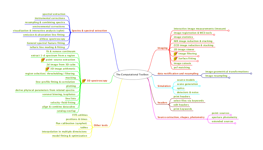
A high-level categorization of the tasks described in this section. Many of the nodes in this map have sub-nodes and sub-sub-nodes that are not shown but would generally comprise separate tools. At the level of detail shown here there are ~50 categories of tools. In the end this will probably expand into of order 103 individual tools.
8.1. General-purpose multi-dimensional Array Analysis tools
The descriptions of the tools here are deliberately brief. The main goal is to highlight the basic functionality. In many cases basic functionality already exists within the various python scientific libraries. In those cases, the development effort for astronomers is generally focused on building interfaces to make them convenient to use on astronomical data sets. This includes:
- Consistent approaches to masking or rejecting data
- Consistent approaches to handling of undefined data and masks
- Consistent approaches to dealing with error arrays and data quality arrays
- Consistent approaches to dealing with metadata, including WCS information
- Consistent approaches to history and logging
8.1.1. Interactive Image Measurements
The new tools need to have the kinds of functionality currently supplied
by IRAF’s imexamine tool. This includes:
- centroids
- contours
- 3d surface plots
- 2d cuts
- localized histograms
- aperture photometry
- basic statistics
8.1.2. Basic Statistics
The includes basic statistics like mean, median, standard deviation, minimum and maximum, with optional masking, setting of a floor and ceiling on input values and rejection of outliers.
8.1.3. Filtering
There is already rich set of image filtering tasks in the scipy ndimage module, the scipy signal and in scikit-image. However, these do not always deal gracefully with image masks, undefined values, or error arrays. The astropy nddata module is aimed at addressing this issue. Filtering includes the following, all in N dimensions, where N is at least 3 for JWST data:
- smoothing
- convolution
- gradient detection
- wavelets
8.1.4. Surface Fitting
A very common operation for astronomical images is to fit a relatively smooth line, surface, or multi-dimensional manifold to a data set (with optional masking and iterative data rejection). This is closely related to smoothing, except that the surface is parametized somehow. The following parametrizations are common enough that they should be provided:
- orthogonal polynomials (e.g. chebyshev)
- splines
8.1.5. Interpolation
There are many, many applications that involve interpolation in dealing with astronomical images. A typical application involves estimating the sky background associated with sources in the image. A set of background estimates from “clean” regions in the image are usually interpolated to the positions of the sources. Another example is in applying geometrical transformations to images. The fluxes on a rectangular pixel grid are used to estimate the fluxes that would have been measured on a different pixel grid.
8.1.5.1. Relatively Certain
The following kinds of interpolation should be included:
- multi-dimensional linear and polynomial interpolation
- spline interpolation
8.1.5.2. Under Consideration
- Inverse distance-weighted interpolation, and variants that use local neighbors
- Natural neighbor interpolation
- Radial basis function) interpolation
- Gaussian processes regression, or Kriging, commonly used in geospatial modeling
- Band-limited interpolation (e.g. sinc or Lanczos)
- Drizzling
8.1.6. Geometric transformations and resampling
The toolbox will include a wide variety of ways to transform images. Many of these involve resampling, and interpolation. Most of the framework for doing this already exists in python numerical libraries. For geometric transformations, easy things should be easy to perform:
- Block averaging or block replicating
- Linear transformations (shift, magnify, rotate, transpose)
Harder things should be possible:
- Affine transformations (preserving straight lines and planes)
- Arbitrary geometric distortions
- Standard map projections (extensive support for various projections exists in matplotlib, but it is currently hard to extract the projected data for other uses).
It is would be useful to make making the different interpolation options easily accessible to the geometric-transformation tools.
8.2. Imaging
In this section, we focus on tools that are mainly needed for undispersed images of astronomical sources. Some of these tools apply to images that are spectrally dispersed as well, but most of those tools are discussed in the spectroscopy section.
8.2.1. Image Registration & WCS Tools
Even if JWST images are perfectly rectified by the standard pipeline, it will be frequently
necessary to register other images to the JWST images. The geometric distortion properties
of these images are sometimes unknown and must be derived using the data themselves.
The various tasks involved (many of which are in the IRAF immatch package) include:
- image distortion fitting
- image rectification
- aligning images
- combining images to a common grid
- matching catalogs (triangle matching)
- image cross-correlation
8.2.2. NIR Image Reduction & Stacking
This would replace the functionality of the IRAF irred package.
8.2.3. CCD Image Reduction & Stacking
This would replace the functionality of the IRAF ccdred package.
8.2.4. Peak Finding
Peak finding is a typical operation on astronomical images. It is the first step of any source detection and photometry package, but is often useful by itself. Routines to do this in scipy and scikit-image would serve as a starting point.
8.2.5. Image Segmentation
Image segmentation is often the next step after finding peaks. Pixels are assigned to sources via some algorithm. The routines for image segmentation in scipy and scikit-image serve as a good starting point. They provide a rich set of options for tasks such as labeling pixels associated with HII regions or clusters within an individual galaxy.
8.2.6. Image Cutouts
Obtaining cutouts of selected sources from a database of larger images is a common operation, but one that has not been standardized. Most organizations serving out data now support the IVOA Simple Image Access Specification (SIAP). However this does not solve the problem of how to organize the data or determine footprints. The IVOA has a draft of a footprint specification open for comments. Many of the institutions serving large data sets support SIAP and are headed toward common standards for footprints. However, tools are needed to help individuals and small groups accomplish the same functions on their smaller datasets for their own use.
8.2.7. PSF Matching
The need to match the point-spread function between different images is very common, and a place where existing tools need improvement. Typically one wants to determine the convolution-kernel that, when applied to a high-resolution image, produces an image with the point-spread function of a lower-resolution image. Examples include matching the PSFs of a JWST NIRCam image to that of a MIRI image. Or matching a JWST image to a ground-based image. The PSF kernel may be spatially varying across the image. Sometimes one has PSF models for each instrument that can be used to construct the PSF kernel. Other times, one must rely on sources in the image, which may or may not be point sources.
A popular algorithm in ground-based astronomy is the Alard-Lupton method of decomposing the kernel into a set of Gaussian basis functions. This is widely used in the supernova-search community. It works very well for typical ground-based PSFs but the Gaussian basis-function may not be the best choice for PSFs with a lot of structure or broad wings. Becker et al. (2012) discuss other methods and promote a method using regularized delta functions. Regardless of the method, the toolbox needs to have efficient, flexible tools for selecting the sources to use for PSF matching, iteratively and perhaps interactively rejecting bad ones, evaluating the results, extracting the kernels, and applying them for photometry or image subtraction.
8.3. Spectra and Spectral Extraction
8.3.1. Spectral extraction
At the simplest level, spectral extraction means turning a two-dimensional dispersed image into a one-dimensional spectrum. This involves separable steps:
- Identifying the pixels to be used for source and background;
- Co-adding the pixels in the cross-dispersion direction according to a specified weighting (and masking) scheme and subtracting background.
Generally speaking, the task of spectral extraction does not include:
- Converting pixels to wavelength
- Converting counts to flux
Nevertheless, there need to be user-oriented tools layered on top of spectral extraction that apply the dispersion solution and flux calibration.
While the JWST pipeline will generally attempt to extract scientifically useful 1D spectra of the objects in the field, it is very likely that astronomers will want to control the extraction in different ways. Some of this can be done by tweaking pipeline parameters, but there also need to be general-purpose tools for doing this driven from parameter files or GUIs or regions on an image display.
This software can become quite complex, depending on the level of sophistication.
A simple approach involves selecting a spectrum on a rectified image (where all spectra are straight lines and where there is a linear wavelength scale per pixel), extracting a rectangular region from this image and summing along columns or rows. This is very useful for quick-look analysis, but often insufficient for the final scientific analysis.
The next level of sophistication selects a curved spectrum on a non-rectified image, where the wavelength scale may not be linear. Either the software traces the spectrum, or has a pre-defined map of the spectral traces so that it can extract the spectrum. It then applies the dispersion solution and either constructs a 1D array with a linear (or logarithmic) relation between wavelength and pixel number, or it constructs a table where each row has a wavelength.
There is also a further level of sophistication, which uses a rectified, co-added image from multiple exposures as a tool by which to identify source and background regions. However, these regions are then transformed back into the reference frame of the original individual (probably dithered) exposures and the spectral extraction is carried out there. This minimizes number of resampling steps carried out on the data and simplifies the propagation of uncertainties.
It is a goal to support all three methods of spectral extraction, with both GUI-specified extraction regions and regions specified via input parameters.
8.3.2. Resampling & combining spectra
Resampling a 1D spectrum can mean taking a spectrum on one wavelength scale and putting it on another scale. Or it can mean taking a table of fluxes and wavelengths and turning it into an array with a specified wavelength scale. Or it can mean taking a model spectrum and interpolating it to find its values at the wavelengths of an observed spectrum. Resampling involves interpolation and is therefore an approximation. There are many different ways to interpolate, each with its own strengths and weaknesses. Many interpolation methods are already supported by scipy and numpy, so the primary goal is to provide interfaces to these interpolation methods so that they can be easily applied to astronomy data sets with attention to metadata, error arrays and masks.
Resampling 2D spectra is more complicated and often requires a detailed specification of the image distortions and wavelength calibrations of the instruments used to obtain the data. At the lowest level it is just 2D interpolation. The main challenge is to develop a simple, yet general mechanism to specify the image geometries.
Combining spectra involves co-adding or finding some robust measure of the mean of data from several different sources. The weights often depend on the uncertainties and masks. The co-added spectra should have associated uncertainties when it is possible to compute them.
8.3.3. Visualization & interactive analysis (splot)
An important functionality for the Graphical User Interface(s) is to provide interactive viewing and manipulation of one-dimensional spectra. The type of functionality needed includes that available in the splot package, SPECVIEW, VOSPEC, the STARLINK SPLAT package or a variety of individually-maintained IDL tools.
Perhaps more important than the specific functionality is to develop a framework to make it easy for astronomers, who are generally not experienced GUI developers, to add functionality to the GUI for a particular science application.
8.3.4. Emission & absorption line fitting
The software tools need to include a variety of fitting functions and fitting methods. Fitting functions should include simple Gaussians and Lorentz and Voit profiles, as well as more elaborate functional forms. The software should allow for convolution with a wavelength-dependent line-spread function. It should provide a variety of minimization routines and ways of treating uncertainties and missing data. It should work well in regimes where the assumption of Gaussian uncertainties on the fluxes is not valid (e.g. for very low counts/pixel). It should have ways to convert the results into physical units. It should be straightfoward to use the same software to assess uncertainties via resampling or Monte-Carlo techniques.
8.3.5. General spectral fitting
In addition to fitting emission and absorption lines, there need to be tools for estimating or fitting continua (used in line-fitting). This includes allowing the user to interactively select regions to use for continuum fitting, as well as providing algorithms for iteratively masking emission and absorption features as part of the determination of the continuum spectrum.
There also need to be tools for fitting heuristic or physical models to spectra, e.g. along the lines of the contributed package specfit in STSDAS.
8.3.6. Line lists
8.3.6.1. Relatively Certain
The toolbox should contain convenient, well-documented lists of the wavelengths of lines commonly seen in astronomical objects.
8.3.7. Slitless spectroscopy
HST and JWST each have two slitless spectrographs. The JWST NIRSpec MOS can also mimic a slitless spectrograph. The lack of a slit creates several challenges for slitless spectroscopy:
- Spectra from several sources can overlap;
- Overlap can include a zeroth-order image or spectra from higher orders;
- Spectra taken at different rotations can be used to overcome some of the effects of blending;
- The wavelength calibration depends critically on knowing the source positions; and
- The convolution kernel for a spectral feature can be quite broad because it not truncated by a slit.
For HST, slitless spectroscopy has been supported by the AxE package. The 3D-HST Treasury Program developed a separate set of tools. Regardless of the ability of the JWST pipeline to meet all the calibration needs, tools for observers to inspect the original 2D spectra and extracted 1D spectra, manipulate and re-run the extraction, model the line-spread function, and deal with the source confusion are essential.
Searches for emission lines (such as Lyman-alpha lines from very distant galaxies) are hopeless without dealing with most of these issues. It would clearly be of interest to observers to have a tool that searches for emission lines in the data automatically, accounting for the difficulties of spectral overlaps and the fact that the S/N for a significant detection is dependent on the size of the line-emitting region and the underlying background due to sky and galaxy continuum.
8.3.8. Instrumental corrections
For JWST and HST, the instrumental corrections are the job of the pipeline. The pipeline parameters and tasks themselves can be modified and re-run by the user. These include:
- converting counts to calibrated fluxes in physical units; applying sensitivity, flat-field and illumination corrections
- converting pixel positions to wavelengths
To the extent that the assumptions for different instruments can be standardized, it would be useful to include the building blocks for applying instrumental corrections for other instruments in the general set of tools. However, because this depends on standardized formats for calibration information, it will require broad community involvement. One way forward would be to develop a prototype of applying insrumental corrections to a popular ground-based spectrograph, using the same calibration philosophy that is used for JWST, and document this as a template for other instruments.
More importantly, there are tasks involved in deriving these corrections that are in common to HST and JWST instrument scientists and the large community of astronomers needing to calibrate other instruments:
- deriving the instrumental sensitivity from standard-star observations;
- deriving the instrumental flat field;
- deriving instrumental illumination corrections;
- deriving the instrumental dispersion solution; and,
- deriving the absolute wavelength calibration
In the case of ground-based observations, some of these calibrations need to be applied night by night, while for the space instruments there is no need to worry about atmospheric variations and other time dependencies (e.g. thermal changes of the instrument) tend to be much slower.
8.3.9. Environmental corrections
It is useful to separate environmental corrections from instrumental corrections, with the distinction that the environmental corrections generally happen outside of the telescope. These include:
- Correcting spectra to heliocentric, galacto-centric or cosmic-flow corrected velocities;
- Shifting spectra to the rest frame;
- Correcting for interstellar reddening and extinction;
- Correcting for scattered light;
- Modeling and/or removing telluric features; and,
- Correcting for airmass and atmospheric extinction
The last couple items on this list are unique to ground-based instruments. The rest are important for JWST and HST, although some of these are done in the pipeline.
8.4. 3D Spectroscopy
In 3D spectroscopy, instead of having a two-dimensional image, the scientist is presented with a three-dimensional image, with two dimensions of spatial information and one dimension of wavelength information. There are some unique challenges to these kinds of data. However, there is also a lot of commonality with 1D and 2D spectroscopy (for example in extracting 1D spectra or fitting spectral features).
For JWST 3D spectra (in NIRSpec and MIRI), an image slicer reorganizes the incoming light to provide non-overlapping spectra of slitlets – small rectangular slices of the sky. These dispersed spectra are collected in a 2D detector and can then be re-assembled into a 3D data cube in the pipeline, after correcting for various distortions in the optical system. Generically, the data-analysis tools allow astronomers to view, select, and analyze data in this 3D space.
It is worth pointing out that this is not the only way of storing the 3D information. It is the most convenient way for a user to view the 3D data, but it involves resampling. Provided one has the tools to map from the original detector reference frame to the rectified 3D image frame, one can imagine developing tools that allow viewing and selection in a rectified 3D image, but do the extraction and analysis on the original pixels. Such tools are more challenging to develop, but are part of the trade space being considered.
In this section, for the sake of brevity, we concentrate mostly on tasks that are specific to the 3D nature of the data. Once one has selected regions to used for the source spectrum and the background, many of the tasks (e.g. fitting spatial or spectral models) are functionally equivalent to the 1D or 2D cases.
8.4.1. 3D image arithmetic, filtering, thresholding, and masking
Basic tools for arithmetic operations on 3D data cubes will be provided. This includes simple operations like add/subtract/multiply/divide as well as applying more complex functions. All of this generic functionality already exists in numpy and scipy, so the development effort will be in developing interfaces that do sensible things with metadata, errors and masks.
The basic tasks for thresholding, masking, peak-finding, convolution, filtering, and general signal processing also mostly exist in the numpy/scipy infrastructure and will not require a huge effort to incorporate into 3D spectroscopy tools.
The standard mechanisms for slicing arrays, doing statitistics, and projecting/summing along dimensions will be available.
8.4.2. Align & combine datacubes
An alarmingly common operation will be to try to align and combine data cubes. This could be to produce spectra of the same sources over a wider spectral range (i.e. combining in the wavelength direction) or to produce co-added spectra of sources taken in separate (possibly dithered) exposures. The JWST pipeline will deal automatically with some of the latter, when the images fall in a pre-defined association. However, users will no doubt want to create their own associations.
If the image alignment is not already known, the tools described in the Imaging section above can be used to align extracted 2D projections of the 3D data cube. If this is shift, rotation and scaling, the alignment can be fairly simple. If it involves geometric distortion, it can be quite complex.
The image combination operation can be challenging. In the wavelength direction, the spectra may overlap and may have different wavelength scales. The user may want to weight the spectra via some algorithm and may want to apply masking. The user will generally want to produce an error array to accomany the combined data dube. These operations almost certainly involve interpolation, and therefore involve some science-specific decisions. The same considerations apply to the spatial dimension, which could in principle include image distortions. The challenge is to create a set of tools that include:
- a simple interface for quicklook or for cases where the exact details of the image combination are unimporant;
- more elaborate interfaces and documentation to allow users to tailor the image alignment and combination to their science goals.
8.4.3. Fit & remove continuum
Fitting and removing a continuum is a generic task that applies to 1D, 2D and 3D spectroscopy. In a 1D spectrum, the astronomer usually specifies regions to use for fitting the continuum – either interactively or via some algorithm that iteratively detects emission and absorption features and masks them out. The fitting algorithm could be parametric, or could involve interpolation. The choice depends on the data and the science application. Tools need to be flexible enough support many options.
The philosophy of region-selection selection in the wavelength dimension is the same for 2D or 3D data, but now the spectra have to be combined somehow either to provide a visual display of a 1D co-added spectrum of a given spatial region to allow the astronomer to select the regions to use (or mask out) in the fitting, or there needs to be a specification of how the iterative masking algorithm averages over the spatial pixels. Sometimes there will be spatial as well as spectral masks (e.g. to remove foreground sources).
In a 1D spectrum there is one continuum spectrum. In the 2D and 3D cases there are more choices to be made. In 2D spectral analysis, there could be a single 1D continuum spectrum that is modulated by the spatial profile of the source, or there could be separate continuum spectra for each pixel in the spatial dimension. The approach depends on the S/N and the science application. Similarly for a 3D data cube, the science and S/N may dictate whether one tries to derive and divide out a single continuum spectrum for all spatial pixels, a continuum spectrum that varies smoothly in some fashion along spatial coordinates (e.g. via fitting or interpolation) or a separate continuum spectrum for each spatial pixel.
8.4.4. Extract 1D spectra from regions
A common operation on 3D data cubes is to extract 1D spectra from specified regions. These regions could be selected:
- interactively on the 3D visualization tool
- via adaptive spatial binning such as Voronoi tesselation
- via thresholds in S/N or isophotes, applied to specific wavelength ranges
- via scripts
- via tables.
These regions can have a variety of shapes, which may or may not be connected. The tools should allow the selection of background regions as well.
The tools should support different ways of combining spectra (e.g. sums, means with and without weighting, or medians). The tools should return error arrays and bad-pixel masks when relevant.
8.4.5. Construct a 2D image from 3D cube
A typical operation on a 3D data cube will be to construct a 2D image of some specific region in wavelength (e.g. emission lines) This operation may include some interpolation over masked pixels in the wavelength dimension, so is not quite as simple as summing along one dimension of a 3D array.
One use of such a projected image is to drive automated algorithms for 1D spectral extraction from the data cube. For example: find peaks in the image, create extraction apertures around those peaks and extract the associated 1D spectra. The same tasks used for peak-finding and image segmentation described earlier in the Imaging section can be used for this.
8.4.6. Point-source extraction
The 1D extraction of the spectra of point sources is a special case.
8.4.6.1. Relatively Certain
The tools should support optimal extraction weighted by the PSF profile, or simple aperture extraction.
8.4.6.2. Under Consideration
More challenging, but possible, is to derive the 1D individual spectra of point-sources in very crowded fields where the PSF wings substantially overlap. This involves simultaneously fitting for the fluxes of the overlapping sources, and results in 1D spectra that have significant covariance with the spectra of their neighbors.
8.4.7. Line-profile fitting & correlation
3D spectroscopy is often used to analyze kinematics. At the root level, this involves extracting and analyzing 1D spectra of spatial regions within the image, but the desired data product returned to the user is generally not a big table of numbers, but rather some more informative visualization. Use cases include:
- Fit a Gaussian to and derive centroids and higher order moments of an emission line profile to derive gas kinematics of emission. The input is a 3-D datacube sub-region. The output is a set of 2-D images that describe the Gaussian fits, and velocity centroid, dispersion and higher order moments of the profile.
- Fit two Gaussian profiles to an emission line profile to derive gas kinematics of emission. The input is a 3-D datacube sub-region. The output is two sets of 2-D images that describe the velocity centroid, dispersion and higher order moments of the profile.
- Fit a user input 1-D spectrum (e.g., instrumental line profile model) to an emission line profile to derive gas kinematics of the emission. The input is a 3-D datacube sub-region and 1-D spectral template. The output is two sets of 2-D images that describe the velocity centroid, dispersion and higher order moments of the profile.
- Correlate the IFU datacube to a template spectrum to generate stellar kinematic diagnostics from absorption line spectra in a continuum source. Inputs are the 3-D datacube region plus a template 1-D spectrum, outputs are 2-D image maps of the velocity and dispersion.
It will clearly be beneficial to have user-friendly GUI-driven tools for this kind of work, layered on top of the simpler tools that do the spectral extraction and fitting.
8.4.8. Interactive 3D data-cube Vizualization
8.4.9. 2D Plotting of 3D data
The 3D-spectroscopy toolbox needs to contain a variety of types of two-dimensional plots. There is a clear need for interactive plots to work with the data-analysis tools themselves. There is also a clear need for publication-quality graphics.
Use cases include:
- Create figures using two 2-D images -– e.g. using a continuum emission image, overplot contours from the other image. User inputs include display levels for image and contour levels and a color table. (This is already largely doable in the current version of DS9, although it could be made more convenient).
- Create a velocity channel map using a 3-D input cube
- Create a 3-D plot view with parameters from the 3D visualzation tool inputs
- Create a figure presenting multiple 2-D images (not linked in velocity) using input from the 3D visualization tool.
- Create a plot with multiple 1-D spectra from the 3D visualization tool.
- Create recipes or canned wrapper macros that permit creation of some of these figures with fewer clicks by the user, and no external saves.
Most of these plot types are easily supported in matplotlib (in both quicklook and publication-quality forms), so the software development can be concentrated primarily on providing the linkage to the 3D visualization tool, and on layers to make use of data models and metadata to put coordinate systems and physical units on the plots.
8.4.11. Velocity-field fitting
8.4.11.1. Under Consideration
A fairly common operation in galaxy research is to fit a velocity field with a model (e.g. tilted disks, with or without constraints on the one-dimensional rotation curve). Ideally, the fitting is done on the ful data cube, but the visualization is on lower-dimensional slices. Tools for such modeling exist, particularly in the radio community. Further investigation is prudent before developing a new tool.
8.4.12. Catalog overlap
Tools should be provided to ingest catalogs and use them to overlay on 3D data cubes or drive spectral extraction.
8.5. Source extraction, morphology and photometry
Various types of source extraction have already been mentioned above in the imaging and spectroscopy sections. The toolbox needs to include well-documented tools for the following:
- Aperture photometry
- PSF construction
- PSF-kernel construction for matching images with different resolution
- Multi-band crowded-field photometry with or without positional and flux priors (incorporating priors is an area of weakness of existing codes).
- Point-source detection in crowded field
- Faint-galaxy source detectection
- Faint-galaxy photometry
- Faint-galaxy morphology
This is an area where very capable tools already exist both inside and outside of IRAF. This includes:
- SExtractor, a stand-alone monolithic C program for faint-galaxy detection and photometry driven by a traditional parameter-file interface.
- GALFIT for fitting parametric models to galaxy images.
- GALAPAGOS A set of IDL scripts that tie together SExtractor and GALFIT.
- DAOPHOT for crowded-field stellar photometry.
- DOLPHOT for crowded-field stellar photometry.
- DOPHOT for crowded-field stellar photometry.
- MATPHOT for crowded-field stellar photometry.
The stellar-photometry codes all take somewhat different approaches to deriving and parametrizing the PSF and fitting the PSF to the crowded images. A version of DAOPHOT exists within IRAF.
Because these are very capable (and complex) codes, there is currently not much urgency in the HST+JWST community to create new codes. That said, many of these codes are maintained by a single person, with no guarantee they will be maintained indefinitely, and there are some limitations of current codes.
In summary, these capabilities are needed whether by ensuring maintenance and interoperability with a existing codes, or developing new tools.
Regardless of whether exiting monolithic packages for doing star and galaxy photometry are supported as part of the toolset for JWST observers, it would be very valuable to provide modular tools for astronomers to experiment with new algorithms. The tools for image filtering, segmentation, and morphology within scipy and scikit-image are already quite powerful, although it is unclear that they would be fast enough for a production environment.
8.6. Simulation
Simulations are absolutely essential for analyzing modern astronomical data. Simulations are the best way to estimate the the flux biases, uncertainties, selection functions, and completeness of samples of stars or galaxies measured in an image or a survey. Typically one would like to either construct purely simulated images with realistic simulations of the S/N, PSF, and instrumental charactiistics, or one would like to insert simulated objects into the real images. To prevent the uncertainties in the analysis from dominating the final uncertainties, one will typically insert many more sources into the images than true sources, but do this a few sources at a time to keep the crowding more or less the same.
In IRAF, simulations have been supported by the ARTDATA, which is flexible and quite fast. This package does not include tools for modeling model instrument characteristics.
A flexible simulation package should include the following:
- Source shapes (point sources, various galaxy models)
- A library of astronomical source spectra
- The ability to apply an instrumental response function to spectra (e.g. pysynphot)
- Distribution functions to describe populations of sources with varying fluxes or spectral properties (e.g. luminosity functions)
- Spatial distribution functions
- At a minimum, the ability to convolve with point-spread functions
- Poisson and Gaussian noise models
Certain aspects of this are already supported by pysynphot, which takes input spectra and instrument throughputs and calculates count rates.
A more sophisticated simulation suite would attempt to model the full effects of the environment, optics, and detector. The LSST Image Simulator, treats each incident photon individually, accounting for the effects of the atmosphere and optics, non-uniformities in the detectors, charge diffusion, etc. Various proprietary simulators exist for the JWST instruments, but there are currently no plans to support these for general observers. Nevertheless, it is important to have reasonably high-fidelity simulations that include the specific characteristics of the instruments in order to develop the JWST pipeline. It takes more effort to develop these for general use, but they would undoubtedly be useful to many observers.
It would also be extremely useful for the simulation suite to provide access various kinds of sky models:
- A Milky Way model for star counts
- A Milky Way model for extinction
- A diffuse sky-background model (including zodiacal light, galactic diffuse emission, and extragalactic background radiation)
- Hertsprung-Russell diagrams and a tool to build stellar populations
- A tool for building synthetic galaxy spectra for an assumed star-formation history and chemical evolution
- Cosmological galaxy-evolution simulations
The situation for these is very similar to that for photometry packages. There are many existing codes that work well and are widely used in the community. There is thus little pressure to create new codes and at least the initial focus should be providing access and interoperability.
8.7. Other tools
This section lists other astronomy-specific tools not mentioned above that will be commonly used. Many of these tools exist in some form in astropy already.
8.7.1. Utilities for reading, writing, and manipulating FITS files and headers
The standard for python has been pyfits for the past few years. This is now incorporated into astropy as astropy.io.fits. In addition to reading, writing, and creating files, it offers standard pythonic ways of accessing the metadata in the image headers.
The equivalent of the following IRAF tasks are needed:
- hselect - select files on disk via header keywords using various boolean operations
- hedit - batch editing of keywords
- eheader - an STSDAS task for editing keywords in emacs or vi
When fits IO is needed in C it will be provided by CFITSIO.
8.7.2. Utilities for reading, writing and manipulating tables
Astronomers deal with tabular data constantly. The storage formats includ ASCII files with various formats, FITS, VO Tables, and databases. For small tables, the routines for manipulating the table and doing operations (plotting statistics, model fitting, etc.) can be independent of the table format once the table is read in. For large data sets that do not fit in memory, this is not as straightfoward.
Various utilities exist within python and astropy for dealing with tabular data, all of which have slightly different purposes:
There is work to be done to improve the convience to astronomers for:
- reading and writting various formats
- dealing with missing data
- dealing with uncertainties
- interpolation (with a rich set of options)
- gridding irregularly sampled data
This is a place where well-designed tools with good documentation and tutorials can save the community a lot of time.
8.7.3. Utilities for dealing with astronomical times and positions
Astropy now includes tools for manipulating world coordinate systems in astropy.wcs. It includes basic functionality for manipulating times and dates in astropy.time. The open-source pyephem packages is well supported and offers utilities for time and position as well as for computing epheremerides of the solar-system bodies and satellites.
8.7.4. Utilities for model fitting and optimization
This section needs work....
Model fitting is an essential part of the toolbox. It is required in many steps of instrument calibration, as well as in the analysis and interpretation of science data. It requires both full-featured GUI interfaces that allow data selection and interactive manipulation of fitting parameters, as well as fast and robust routines that can be used repeatedly in fitting large data sets.
The tool set should certainly include various kinds of standard functions such as Gaussians and polynomials. Within IRAF there are ~80 different tasks that involve fitting, from general curve and surface fitting like curfit, polyfit and imsurfit, to more specialized routines for fitting continuum in spectra, fitting sky background, fitting standard-star photometry, or fitting ellipses.
The scipy optimize package includes a variety of optimization options. Eric Tollerud, one of the founders of astropy, has provided a somewhat higher level framework for model fitting, including a customized GUI in PyModelFit.
There are a couple of python versions of Craig Markwardt’s popular IDL fitting library.